I gave a guest lecture at Columbia Business School last week: one hour on recommendation systems, for business students. The pitch was simple. Recommenders aren’t a side feature. A model picks the 10 items you see out of a billion, and the business depends on which 10.
Netflix has said about 80% of watched hours come from recommendations (Gomez-Uribe & Hunt, 2015). YouTube’s CPO put their number at 70% of watch time in 2018. Amazon’s often-quoted 35% of revenue is a McKinsey estimate, not something Amazon confirmed. The exact numbers matter less than the shape: on most consumer products, the feed is the product.
The full deck is linked at the bottom. This is the short version.
Learning to rank
Order, not labels
When you start learning ML, you learn regression and classification. A recommender does neither. The question isn’t “will Ana like this item.” It’s “of these 10,000 items, which 10 go at the top, and in what order.”
Three ways to set that up:
- Pointwise: one item at a time — will Ana click this? Simple, but it ignores that items compete for the same slot.
- Pairwise: did Ana prefer A over B? This matches the data you actually have, clicked versus skipped, and it’s where most production systems ended up. LambdaMART, which ran Bing, Yandex, and Airbnb search for a decade, is boosted trees with a pairwise loss.
- Listwise: is this top 10 better than that one? It optimizes what you actually measure. It’s also the hardest to train.
One trap with pairwise data: it comes from “clicked item versus the item above it that was skipped.” Users click the top thing partly because it’s on top. That position bias is part of why the offline numbers lie to you later.
What goes in
Three kinds of features:
- Behavior: counts and rates — how often has this user clicked this item, this category, what’s this item’s conversion rate.
- Content: user and item attributes — age, country, genre, price.
- Context: the request — device, time of day, where in the app.
One training row per (user, item, context) shown, label: did they click. A boosted tree learns the splits; output is p(click). Score every candidate, sort, show the top.
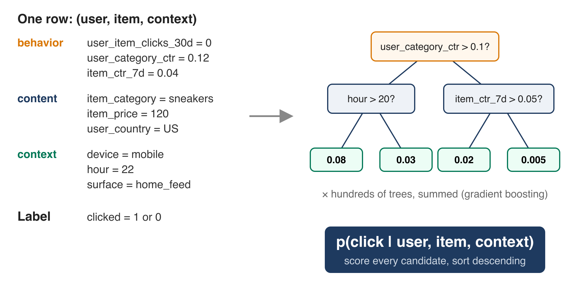
One training row per (user, item, context), through a boosted tree, out comes p(click).
In a mature system, behavior features do most of the work. Honestly, most of the engineering in a recsys team is the pipeline that keeps those rolling counts fresh, not the model.
How you know it’s good
A pointwise model is trained as a classifier, so AUC and log loss tell you whether p(click) is a good probability. But the product is a list, not a probability. So the metrics that matter are ranking metrics: Precision@K, Recall@K, NDCG — a click at position 1 counts more than a click at position 10. And the protocol is always the same: hold out the last week, score it. No peeking at the future.
Serving recommendations
Why a funnel
The simplest system scores every item, sorts, shows the top. At 20,000 titles it’s already too slow. At a billion posts it’s absurd.
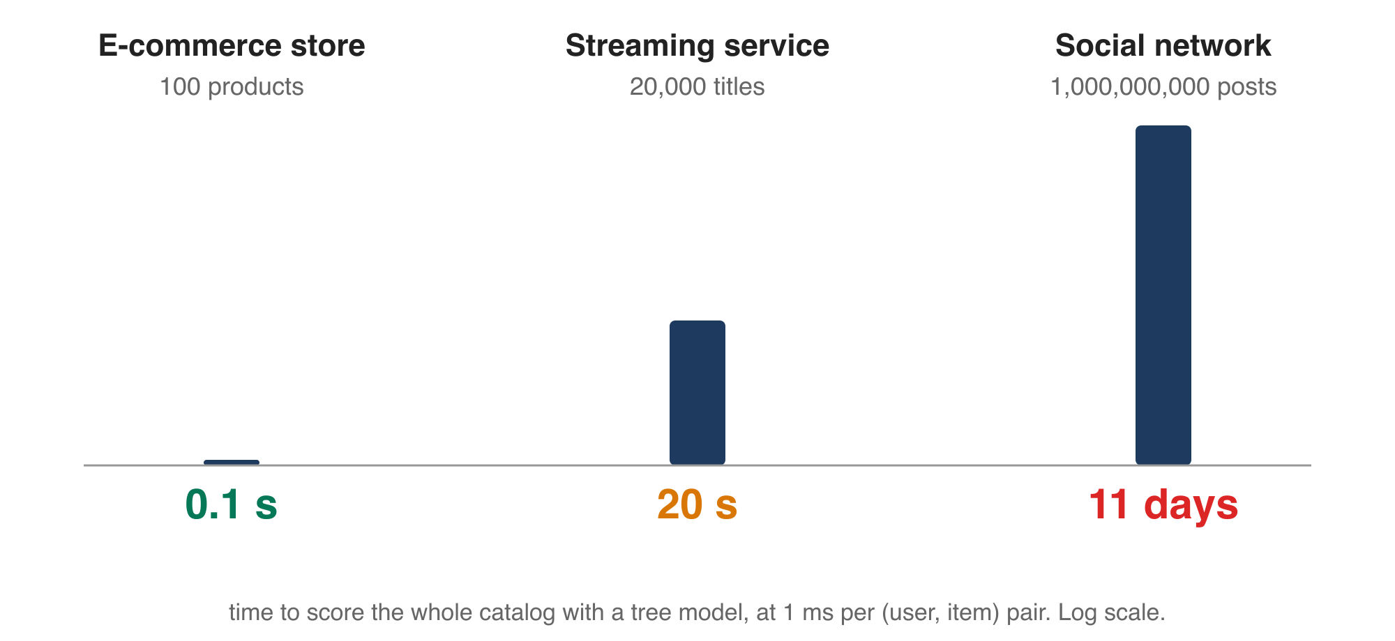
Time to score the whole catalog with a tree model, at 1 ms per pair. Log scale.
A page load is a few hundred milliseconds. So every production recommender at scale is an approximation of “score everything” under a latency and cost budget: relevance, latency, cost — you can’t max all three. Every industry arrived at the same design independently: a funnel, where retrieval gathers candidates cheaply, filtering removes what can’t or shouldn’t be shown, scoring runs the ranking model on the survivors, and ordering turns scores into a page.
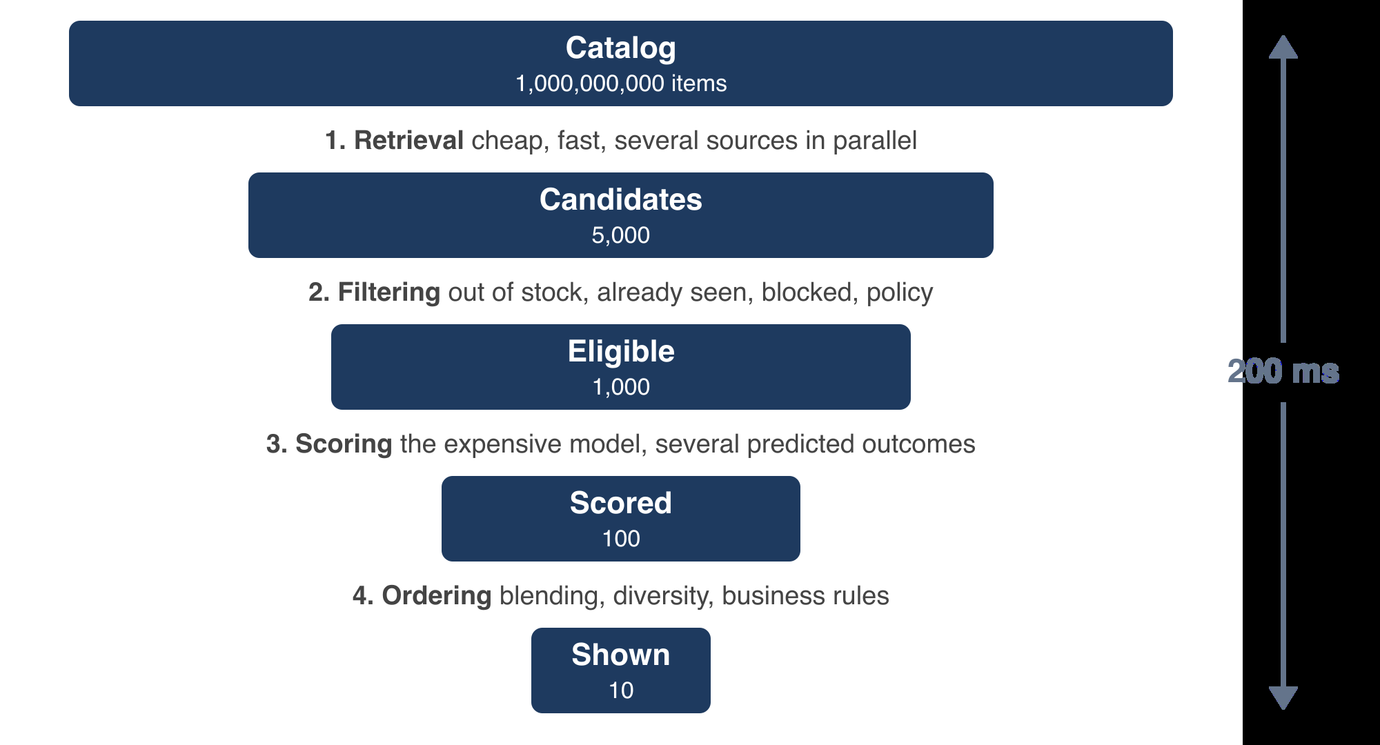
The funnel: a billion items in, ten shown, in about 200 ms.
Search is the same system with a query as one more input. That’s why search and recommendation teams usually end up merged.
Retrieval
Retrieval can afford to be wrong, because the scorer gets a second look. Its job is just: don’t miss anything the scorer would have loved. So it runs several sources in parallel — collaborative (items people with similar behavior liked), content (items whose attributes match), heuristics (new, trending, followed). Any single retriever has blind spots: collaborative reinforces what’s already popular, content never surprises you.
The way collaborative retrieval works at scale: give every user and every item a point in the same space. Close means similar. Ana sits near Oppenheimer and Moneyball, so those are what we retrieve for her. Nobody labels the axes — they come out of the data. In production it’s 64 to 512 dimensions, and retrieval is just: find the nearest thousand out of a billion, approximately, in a few milliseconds (FAISS, HNSW, Pinecone, pgvector — the same tech behind RAG for LLMs). The points come from factoring the interaction matrix: one vector per user and item, chosen so their dot product predicts clicks. The Netflix Prize method, 2009.
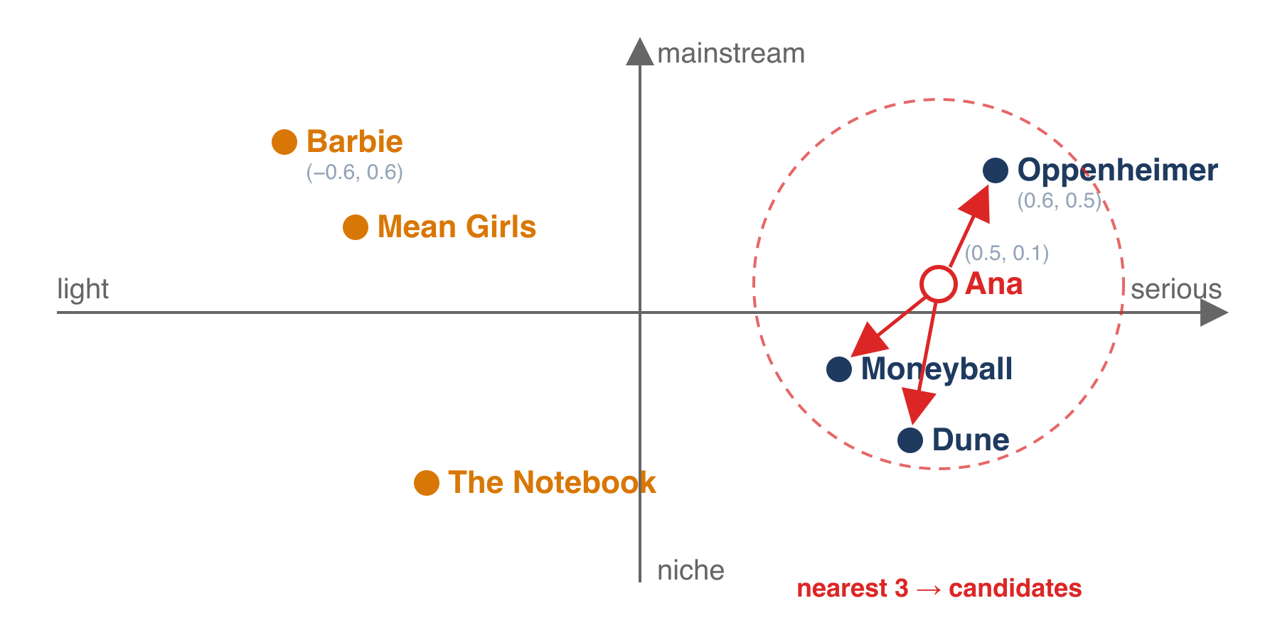
Ana’s nearest neighbors become her candidates.
Scoring
Scoring only has to rank the thousand candidates that survived, so it can afford to be heavy. But one prediction isn’t enough — clicks aren’t the only thing the business cares about. A click that bounces is worth less than a 30-second watch; a purchase is worth more than both; a report is negative. And rare outcomes like purchases (maybe 0.1% of impressions) have too little signal alone. So one shared model predicts several outcomes at once — multi-task learning — and the common ones (clicks) help learn the rare ones (buys).
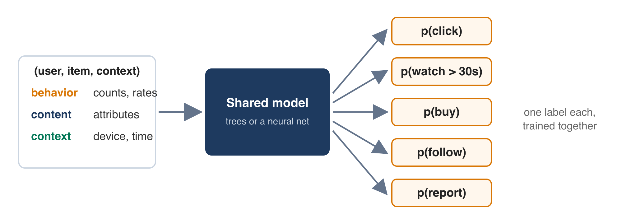
One shared model, one head per outcome, trained together.
Five predictions per candidate, one number to sort by. So you take a weighted sum. The model gives you the p’s. The w’s come from product and leadership — and they encode what the business wants more of. Which means the weights are the strategy, and they’re a decision someone has to own. At Meta, each team was measured on one objective, so a change that raised shares usually cost likes, and both teams ran the same A/B test and reached opposite conclusions. In practice, the loudest voice won. If nobody owns the weights, they get decided by whoever argues hardest.
Ordering
The scorer is pointwise: every item gets a score on its own, with no knowledge of what else is on the page. So the top 5 by score can be five colors of the same shoe. The ordering stage fixes this with rules the scorer can’t express: spread brands, cap duplicates, reserve a slot for new sellers. Total score goes down, the page gets better. In the A/B test, the diverse page usually wins.
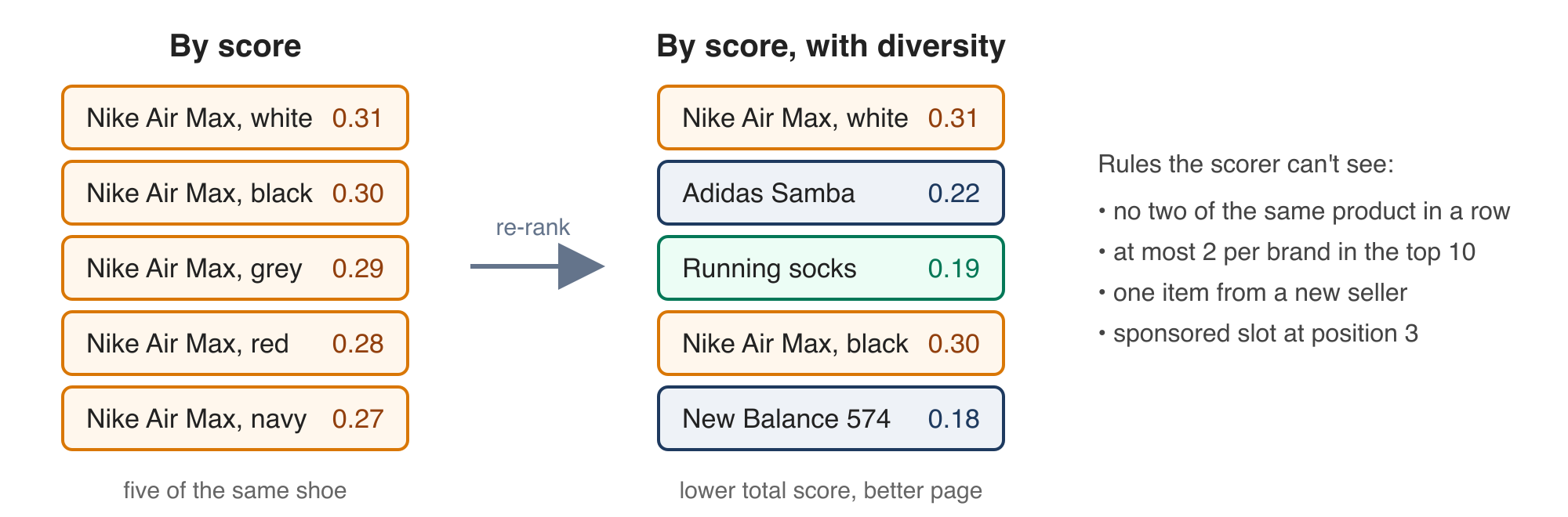
By score: five of the same shoe. With diversity rules: lower total score, better page.
Ordering also handles exploration: deliberately giving up a slot to something uncertain — a new item, one the model has low confidence in, something outside the user’s usual pattern. It costs a little engagement on that slot. It’s also the only way the system learns anything it doesn’t already know. Without it, the loop closes: a user interacts with one partisan post, the model shows more, and after a few months the feed is one-sided. Nobody designed this. It’s what a model trained on its own outputs does by default.
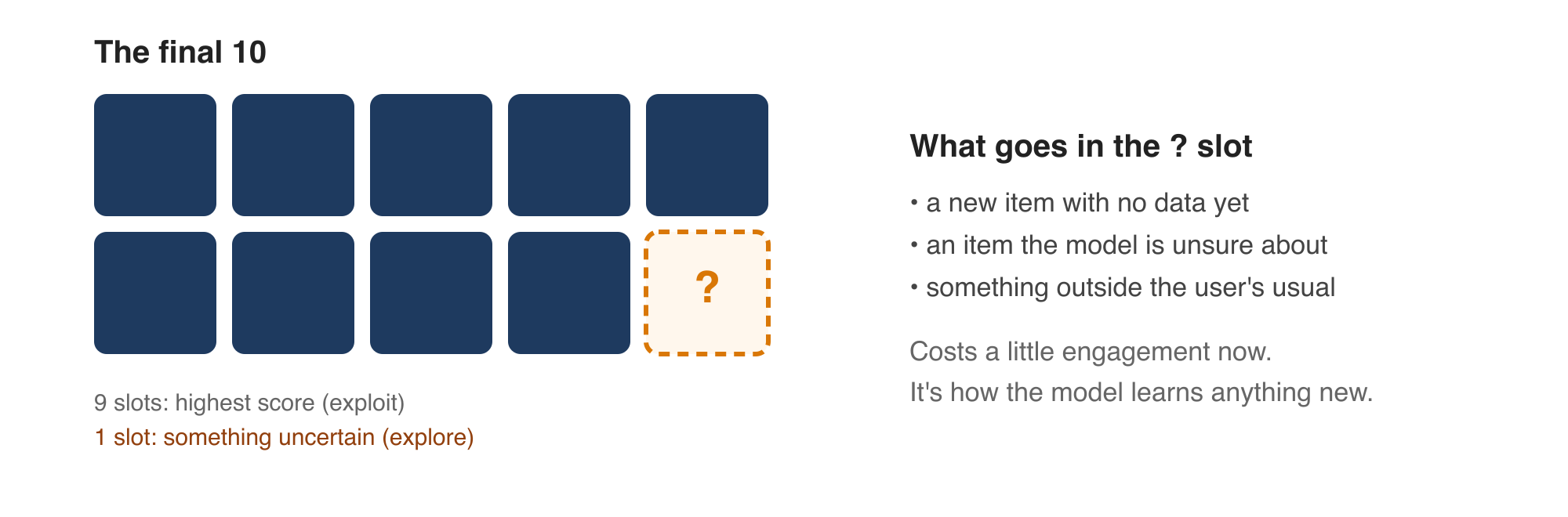
Nine slots exploit, one slot explores. That’s how the model learns anything new.
Evaluating recommenders
Offline isn’t online
Offline evaluation is fast — temporal holdout, ranking metrics — so every model change gets one. The A/B test is the real measure: randomize users, ship to a slice, compare the business outcome. Slow and expensive, so you only run it on candidates that won offline. The problem: offline wins and online wins disagree more often than anyone expects. Two reasons. The metric isn’t the goal: at a news aggregator for developers, optimizing clicks surfaced clickbait — click-through went up and sessions got shorter. And the test data is biased: the holdout only contains what the previous model chose to show, so a model leaning into popularity scores well against it and says nothing about live performance. In about half my projects, offline did not map to online at all.
Two-sided platforms break the test
On a two-sided platform, users affect each other, and a pointwise model can’t see it. The offline metric misses the effect on everyone else, and the A/B test is contaminated because both arms draw on the same supply. Sharpest version: auctions clear at the second-highest bid, so spreading viewers into thin auctions scores worse offline and makes more money. And suppliers who get no demand leave — today’s recommendations decide next month’s supply. On a marketplace, that means 7–14 day user-split tests often can’t resolve a real change. What we do instead: an offline simulator of buyer and seller interactions, longer tests (30–60 days), and cluster randomization, where whole groups of users and sellers are assigned together. The standard A/B test is the starting point, not the answer.
Three things to remember
- It’s a problem about order, not labels. Pointwise, pairwise, listwise.
- The weights are the strategy. The model predicts several things. People choose how to combine them.
- Offline accuracy is not the goal. The metric isn’t the business. Check that offline wins become online wins.
Slides from the lecture are here.